`cmocean` documentation

The cmocean function returns perceptually-uniform colormaps generated by Kristen Thyng. A detailed description of the cmocean project is available at http://matplotlib.org/cmocean.

If you find an occasion to cite these colormaps for any reason, or if you just want some nice beach reading, check out the following paper from the journal Oceanography:

Kristen M. Thyng, Chad A. Greene, Robert D. Hetland, Heather M. Zimmerle, and Steven F. DiMarco (2016). True colors of oceanography: Guidelines for effective and accurate colormap selection. Oceanography, 29(3), 10. doi:10.5670/oceanog.2016.66

Syntax

cmocean
cmap = cmocean('ColormapName')
cmap = cmocean('-ColormapName')
cmap = cmocean(...,NLevels)
cmap = cmocean(...,'pivot',PivotValue)
cmap = cmocean(...,'negative')
cmocean(...)

Description

cmocean without any inputs displays colormap options.

cmap = cmocean('ColormapName') returns a 256x3 colormap. ColormapName can be any of of the following:

cmap = cmocean('-ColormapName') a minus sign preceeding any ColormapName flips the order of the colormap.

cmap = cmocean(...,NLevels) specifies a number of levels in the colormap. Default value is 256.

cmap = cmocean(...,'pivot',PivotValue) centers a diverging colormap such that the point of color divergence corresponds to a specified value and maximum extents are set using current caxis limits. If no PivotValue is set, 0 is assumed. Early versions of this function used 'zero' as the syntax for 'pivot',0 and the old syntax is still supported.

cmap = cmocean(...,'negative') inverts the lightness profile of the colormap. This can be useful particularly for divergent colormaps if the default white point of divergence gets lost in a white background.

cmocean(...) without any outputs sets the current colormap to the current axes.

Examples

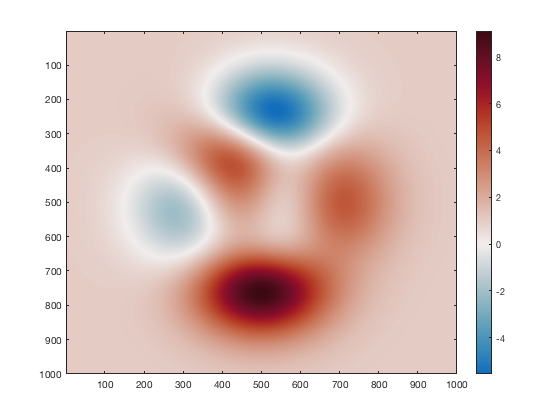
Using this sample plot:

imagesc(peaks(1000)+1)
colorbar

Set the colormap to 'algae':

cmocean('algae')

Same as above, but with an inverted algae colormap:

cmocean('-algae')

Set the colormap to a 12-level 'solar':

cmocean('solar',12)

Get the RGB values of a 5-level thermal colormap:

RGB = cmocean('thermal',5)

RGB =
    0.0156    0.1382    0.2018
    0.3366    0.2317    0.6123
    0.6893    0.3727    0.5097
    0.9772    0.5740    0.2578
    0.9090    0.9822    0.3555

Some of those values are below zero and others are above. If this dataset represents anomalies, perhaps a diverging colormap is more appropriate:

cmocean('balance')

It's unlikely that the center value of this color axis 1.7776 is an interesting value about which the data diverges. If you want to center the colormap on zero using the current color axis limits, simply include the 'pivot' option:

cmocean('balance','pivot',0)

Absolute quantities versus anomalies

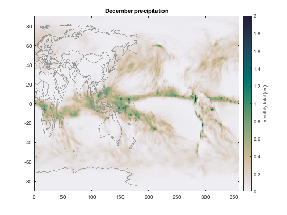
When plotting a linear quantity such as total precipitation in a month, use a linear colormap that goes from light-to-dark or dark-to-light. Here's December 2017 precipitation plotted with the rain colormap:

filename = 'ERA_Interim_2017.nc';
lat = ncread(filename,'latitude');
lon = ncread(filename,'longitude');
tp = ncread(filename,'tp'); % total precipitation

figure
h = imagescn(lon,lat,tp(:,:,12)'*100);
title 'December precipitation'
cb = colorbar;
ylabel(cb,'monthly total (cm)')
cmocean rain

hold on
borders('countries','color',rgb('gray'))
caxis([0 2])

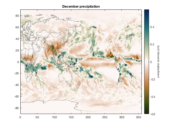
However, anomalies warrant a different approach. Use a divergent colormap to show spatial patterns of anomalies, providing a clear delineation between regions where values are anomalously high, low, or nearly in balance.

Here's the divergent tarn colormap showing December precipitation relative to the annual mean:

Precip_anomaly = tp(:,:,12) - mean(tp,3);

figure
imagescn(lon,lat,Precip_anomaly'*100)
title 'December precipitation'
cb = colorbar;
ylabel(cb,'precipitation anomaly (cm)')
cmocean tarn
caxis([-1 1]*0.6)

hold on
borders('countries','color',rgb('gray'))

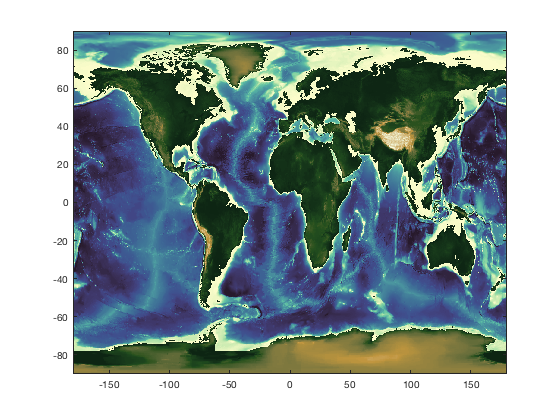
Topography

Topography is a special case because it's usually important to clearly distinguish between land and ocean, but we still want a linear relationship between the perceived color and elevation. A typical divergent colormap like balance or curl might draw the eye toward the general direction of coastlines, but would not provide a clear definition between land and ocean, so the cmocean colormaps include 'topo', which is designed specifically for topography.

[Lat,Lon] = cdtgrid(0.25);
Z = topo_interp(Lat,Lon);

figure
imagescn(Lon,Lat,Z)

caxis([-1 1]*6000)
cmocean topo

Negative colormaps

I was recently in a situation where I had a scatter plot of divergent data on a white background, but cmocean('balance') made the most important datapoints white and nearly invisible. Here's the situation:

% Some sample data with noise:
x = 10*rand(300,1)-5;
noise = 2*randn(size(x));
y = x.^2+noise;

% A theoretical perfect x^2 line:
x_theoretical = linspace(min(x),max(x),50);
y_theoretical = x_theoretical.^2;

% Plot the data:
figure
plot(x_theoretical,y_theoretical,'k-')
hold on
scatter(x,y,25,noise,'filled')
cb = colorbar;
ylabel(cb,'error relative to theory')
box off
axis tight

I wanted to show how far off my noisy data was from the perfect theoretical x-squared line, so the divergent cmocean('balance') map seemed appropriate:

cmocean('balance','pivot',0)

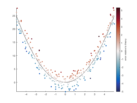
But in the plot above, attention is drawn away from the theoretical line toward the dark red and dark blue outliers. In this case, a negative colormap may be preferred:

cmocean('balance','pivot',0,'negative')

Author Info

This function was written by Chad A. Greene of the Institute for Geophysics at the University of Texas at Austin (UTIG), June 2016, using colormaps created by Kristen Thyng of Texas A&M University, Department of Oceanography. More information on the cmocean project can be found at http://matplotlib.org/cmocean. Updated with new colormaps rain, topo, diff, and tarn in January 2019.

cmocean documentation

Contents