spei_documentation
The spei function calculates the standardised precipitation-evapotranspiration index based on a standardization of a simplified water balance based on the climatology of a particular location.
See also: pet.
Back to Climate Data Tools Contents.
Contents
Syntax
s = spei(t,prec,pevap)
[s,tint] = spei(t,prec,pevap,'integrationtime',months)
Description
s = spei(t,prec,pevap) computes the standardised precipitation-evapotranspiration index s, given precipitation prec and potential evaporation pevap corresponding to times t. prec and pevap can be either be 1D vectors or 3D cubes, whose first two dimensions are spatial and whose third dimension corresponds to times t. The dimensions of prec and pevap must agree. Times t can be datetime or datenum format.
[s,tint] = spei(t,prec,pevap,'integrationtime',months) integrates over 1, 2, 3, 4, 6, or 12 months. The default integration time is 1 month. Output tint contains the dates of the reduced time series.
Example
This example demonstates how to calculate and display temporal and spatial patterns of the standardised precipitation-evapotranspiration index SPEI. We will use NCEP/NCAR reanalysis data (Climate Data Assimiliation System I Daily) downloaded from IRI/LDEO Climate Data Library of the University of Columbia.
The file ncep-ncar.mat contains a number of three dimensional arrays of daily values of mean temperature (T), maximum temperature (TMAX), minimum temperature (TMIN) and precipitation (P) as well as a vectors for time, latitude and longitude. Retrieving these variables from the Climate Data Library is explained at the bottom of this page.
load ncep-ncar
Our data spans following time range
disp([min(t) max(t)])
disp(years(max(t)-min(t)))
   2008-01-01   2018-12-31
   10.9982
Precipitation comes in units kg^2/m^2/s and we change these units to mm/day. Temperatures are in K and we change them to degrees C.
P    = P*3600*24;
T    = T-273.15;
TMAX = TMAX-273.15;
TMIN = TMIN-273.15;
Calculate extraterrestrial solar radiation
Hargreaves and Samani's PET equation requires extraterrestrial radiation (Ra) as input. Ra is the solar radiation on a horizontal surface at the top of the Earth's atmosphere and is computed based on the orbital parameters of the Earth which are dependent on latitude. We wish to have the temporal variations of solar radiation integrated over daily time intervals which can be calculated using the function solar_radiation function. Use meshgrid to turn the lat,lon vectors into grids, which will thereby give us a distinct latitude value for each grid cell:
[Lon,Lat] = meshgrid(lon,lat);

Ra  = solar_radiation(t,Lat);

% Plot grid cell 5,5:
plot(t,squeeze(Ra(5,5,:)))
ylabel('Ra [MJ m^2 day^{-1}]')
title(['Solar radiation at ' num2str(lat(5)) '\circN'])

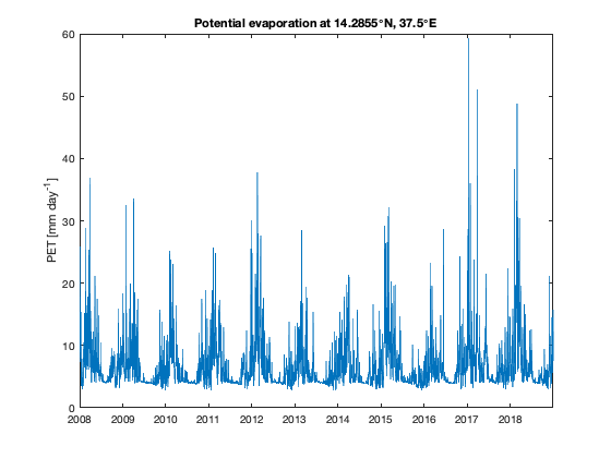
Calculate potential evapotranspiration
SPEI requires precipitation and potential evapotranspiration (PET). PET is calculated based on the formula of Hargreaves and Samani (1985) which estimates reference crop evapotranspiration based on temperature and extraterrestrial radiation.
There are numerous approaches to calculating potential evaporation. A compilation is found here (see supplements). Here we use the formula of Hargreaves-Samani (1985) which is a temperature based method to calculate the potential evapotranspiration (PET) and is implemented in the function pet. The main advantage of using the Hargreaves-Samani equation lies in its simplicity and low requirements regarding input parameters.
pevap = pet(Ra,TMAX,TMIN,T);

plot(t,squeeze(pevap(5,5,:)))
ylabel('PET [mm day^{-1}]')
title(['Potential evaporation at ' num2str(lat(5)) '\circN, ' num2str(lon(5)) '\circE' ])
Calculate SPEI
The SPEI is a drought index that can be used by different scientific disciplines to detect, monitor and analyze droughts. The SPEI allows comparison of drought severity through time and space, since it can be calculated over a wide range of climates. The function spei calculates the index based on the difference between precipitation and PET and enables setting differently sized integration times.
% Two ways of calculating SPEI:
s = spei(t,P,pevap);
[s3,t3] = spei(t,P,pevap,'integrationtime',3);

figure
subsubplot(2,1,1)
plot(t,squeeze(s(5,5,:)))
hold on
plot(t3,squeeze(s3(5,5,:)))
ylabel('SPEI')
axis tight
title(['SPEI at ' num2str(lat(5)) '\circN, ' num2str(lon(5)) '\circE' ])
legend('raw','3 month integration')

subsubplot(2,1,2)
plot(t,squeeze(P(5,5,:)))
ylabel('precipitation [mm day^{-1}]')
set(gca,'yaxislocation','right')
axis tight

Retrieving NCEP/NCAR reanalysis data
Here is the script that shows how to receive the ncep-ncar.mat file that we used in this file.
  whitespace = '%20';
  bopen      = '%28';
  bclose     = '%29';
  datestart = '1 Jan 2008';
  dateend   = '31 Dec 2018';
  lonlims   = '30.0/50.0'; %'27.1875/45.9375';
  latlims   = '20.0/5.0';
  vars      = {'temp','maximum','minimum'};
for r = 1:numel(vars)
url = ['https://iridl.ldeo.columbia.edu/SOURCES/.NOAA/.NCEP-NCAR/.CDAS-1/.DAILY/' ...
'.Diagnostic/.above_ground/',...
'.' vars{r} '/T/'...
'(' datestart ')(' dateend ')RANGEEDGES/' ...
'X/' lonlims '/RANGEEDGES/'...
'Y/' latlims '/RANGEEDGES/dods']; url = replace(url,' ',whitespace);
url = replace(url,'(',bopen);
url = replace(url,')',bclose);
if r == 1
lon = ncread(url,'X');
lat = ncread(url,'Y');
t = ncdateread(url,'T');
end if r == 1
T = ncread(url,'temp');
elseif r == 2
TMAX = ncread(url,'temp');
else
TMIN = ncread(url,'temp');
end
end
T = squeeze(T);
TMAX = squeeze(TMAX);
TMIN = squeeze(TMIN); vars = 'prate'; % in kg/m2/s
url = ['https://iridl.ldeo.columbia.edu/SOURCES/.NOAA/.NCEP-NCAR/.CDAS-1/.DAILY/' ...
'.Diagnostic/.surface/',...
'.' vars '/T/'...
'(' datestart ')(' dateend ')RANGEEDGES/' ...
'X/' lonlims '/RANGEEDGES/'...
'Y/' latlims '/RANGEEDGES/dods'];
url = replace(url,' ',whitespace);
url = replace(url,'(',bopen);
url = replace(url,')',bclose);
lonp = ncread(url,'X');
latp = ncread(url,'Y');
P = ncread(url,'prate');
P = squeeze(P);% The three dimensional arrays have their first and second dimensions switched. % Here we use the function permute to swap the dimensions: lon = lon'; T = permute(T,[2 1 3]); TMAX = permute(TMAX,[2 1 3]); TMIN = permute(TMIN,[2 1 3]); P = permute(P,[2 1 3]);
save ncep-nacar.mat
References
- Hargreaves, George H., and Zohrab A. Samani. "Reference crop evapotranspiration from temperature." Applied Engineering in Agriculture 1.2 (1985): 96-99. doi:10.13031/2013.26773.
- McMahon, T. A., et al. "Estimating actual, potential, reference crop and pan evaporation using standard meteorological data: a pragmatic synthesis." Hydrology and Earth System Sciences 17.4 (2013): 1331-1363. doi:10.5194/hess-17-1331-2013.
Author Info
This function and supporting documentation were written by José Delgado and Wolfgang Schwanghart (University of Potsdam), February 2019, for the Climate Data Toolbox for Matlab.