wmean documentation
The wmean function computes the weighted average or weighted mean value.
Back to Climate Data Tools Contents
Contents
Syntax
M = wmean(A,weights)
M = wmean(...,'all')
M = wmean(...,'dim',dim)
M = wmean(...,'nanflag')
Description
M = wmean(A,weights) returns the weighted mean of the elements of A along the first array dimension whose size does not equal 1. Dimensions of A must match the dimensions of weights.
- If A is a vector, then wmean(A,weights) returns the weighted mean of the elements.
- If A is a matrix, then wmean(A,weights) returns a row vector containing the weighted mean of each column.
- If A is a multidimensional array, then wmean(A,weights) operates along the first array dimension whose size does not equal 1, treating the elements as vectors. This dimension becomes 1 while the sizes of all other dimensions remain the same.
M = wmean(...,'all') computes the weighted mean over all elements. (Requires Matlab R2018b or later.)
M = wmean(...,'dim',dim) returns the mean along dimension dim. For example, if A is a matrix, then wmean(A,weights,'dim',2) is a column vector containing the weighted mean of each row.
M = wmean(...,'nanflag') specifies whether to include or omit NaN values from the calculation for any of the previous syntaxes. wmean(A,weights,'includenan') includes all NaN values in the calculation while wmean(A,weights,'omitnan') ignores them.
Example 1: 1D array
Here's an array of values y and their mean without any special weighting:
y = 0:2:10
mean(y)
y =
  Columns 1 through 5
             0          2.00          4.00          6.00          8.00
  Column 6
         10.00
ans =
          5.00
The answer above is equivalent to using wmean with equal weights for each value in y:
weight = [1 1 1 1 1 1];

wmean(y,weight)
ans =
          5.00
But perhaps you're doing a calculation in which the values close to zero are to be weighted most heavily, like this:
weight = logspace(1,0,6)

wmean(y,weight)
weight =
  Columns 1 through 5
         10.00          6.31          3.98          2.51          1.58
  Column 6
          1.00
ans =
          2.61
Example 2: 2D matrix
Here's a 2D matrix A, and just like in Example 1 we'll start by using equal weights across the board:
% A data matrix:
A = [0 1 2
     2 3 4
     4 5 6
     6 7 8]

% Equal weights everywhere:
w = ones(size(A))

wmean(A,w)
A =
             0          1.00          2.00
          2.00          3.00          4.00
          4.00          5.00          6.00
          6.00          7.00          8.00
w =
          1.00          1.00          1.00
          1.00          1.00          1.00
          1.00          1.00          1.00
          1.00          1.00          1.00
ans =
          3.00          4.00          5.00
If you need to operate across rows instead of down the columns of A, specify dimension 2 as follows:
wmean(A,w,'dim',2)
ans =
          1.00
          3.00
          5.00
          7.00
If you're following along at home, you can prove to yourself that the answer above, in which all weights are equal, gives the same answer as mean(A,2).
Question: How could we make the weighted mean of A turn out to be equal to the second row of A?
Answer: I can think of two ways. One way is to set all the weights to zero, except row 2. Alternatively, we could keep those rows the way they are, and instead set the second row of weights to some insanely large number:
w(2,:) = 1e100

wmean(A,w)
w =
          1.00          1.00          1.00
 10000000000000000159028911097599180468360808563945281389781327557747838772170381060813469985856815104.00 10000000000000000159028911097599180468360808563945281389781327557747838772170381060813469985856815104.00 10000000000000000159028911097599180468360808563945281389781327557747838772170381060813469985856815104.00
          1.00          1.00          1.00
          1.00          1.00          1.00
ans =
          2.00          3.00          4.00
What if one element in A is NaN?
A(2,2) = NaN

wmean(A,w)
A =
             0          1.00          2.00
          2.00           NaN          4.00
          4.00          5.00          6.00
          6.00          7.00          8.00
ans =
          2.00           NaN          4.00
We can ignore that missing entry instead of turning the whole solution for that column to NaN:
wmean(A,w,'omitnan')
ans =
          2.00          4.33          4.00
Example 3: Area-weighted SST
Here's a map of sea surface temperatures using some example data that comes with CDT:
% Load the sample data:
load global_sst

% Convert from Kelvin to Celsius:
sst = sst-273.15;

% Plot SSTs:
imagescn(lon,lat,sst)
cmocean thermal % colormap
cb = colorbar;
ylabel(cb,'sea surface temperature \circC')
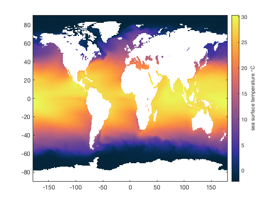
A beginner might try to get the average global sea surface temperature by taking the unweighted mean of all sst values:
mean(sst,'all','omitnan')
ans =
         13.84
However, we must recall that the sst grid corresponds to equally spaced latitudes and longitudes, which are not all equal in area. Lines of longitude converge at the poles, so an area-averaged measure of SST requires weighting the mean by are of each grid cell.
To accomplish this, turn the lat and lon arrays into grids and use cdtarea to get the area of each grid cell. Here are the areas of each grid cell:
% turn lat,lon arrays into grids:
[Lon,Lat] = meshgrid(lon,lat);

% Get the area of each grid cell:
A = cdtarea(Lat,Lon,'km2');

imagescn(lon,lat,A)
hold on
borders % national borders

cb = colorbar;
ylabel(cb,'grid cell area (km^2)')
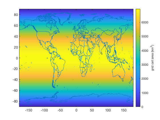
With the grid cell areas A, we can now get the area-averaged sea surface temperature with wmean:
wmean(sst,A,'all','omitnan')
ans =
         18.45
That's quite a difference from the 13.8 degree value we obtained using the unweighted mean! And it's not surprising: The "unweighted" mean in this context was actually a misnomer because by giving equal weight to each grid cell in the mean SST calculation, we were actually giving undue weight to the tiny grid, cold grid cells near the poles. So it is no surprise that the "unweighted" mean SST value is lower than the area-averaged SST value.
Author Info
This function is part of the Climate Data Toolbox for Matlab. The function and supporting documentation were written by Chad A. Greene of the University of Texas at Austin.