`topo_interp` documentation

The topo_interp function interpolates elevation relative to sea level at any geographic points. The data are from the ETOPO5 world digital elevation model, which is provided at 5-minute (or 1/12 degree) grid resolution.

Back to Climate Data Tools Contents

Syntax
Description
Example 1: A grid
Example 2: An elevation profile
Example 3: Load the raw data
Example 4: The effects of sea level rise
A note on aliasing
Author Info

Syntax

zi = topo_interp(lati,loni)
zi = topo_interp(lati,loni,'method',InterpMethod)

Description

zi = topo_interp(lati,loni) returns elevations relative to sea level at the geographic points lati,loni.

zi = topo_interp(lati,loni,'method',InterpMethod) specifies an interpolation method and can be any method accepted by interp2. Default method is 'linear'.

Example 1: A grid

Here's a global grid at 0.25 degree resolution:

[lat,lon] = cdtgrid(0.25);

Elevations at each grid point are obtained like this:

Z = topo_interp(lat,lon);

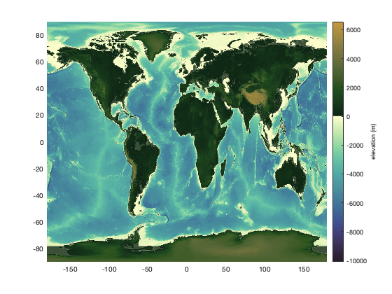
Plot the elevation grid like this. Below I'm using cmocean for the topography colormap:

pcolor(lon,lat,Z)
shading interp

cb = colorbar;
ylabel(cb,'elevation (m)')
cmocean('topo','pivot') % sets the colormap

Example 2: An elevation profile

Suppose you want to take a trip from Paris (48.8567N, 2.3508E)to Bangkok (13.7525N, 100.494167E). Here's a crude line made up of 1000 points between the two cities:

lat = linspace(48.8567,13.7525,1000);
lon = linspace( 2.3508,100.494167,1000);

hold on
plot(lon,lat,'r-','linewidth',2)

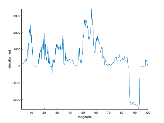
An elevation profile along that route is this easy:

z = topo_interp(lat,lon);

figure
plot(lon,z)
axis tight
box off
xlabel 'longitude'
ylabel 'elevation (m)'

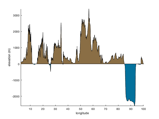
Or to depict the land and water more intuitively, use the anomaly function and specify colors using rgb:

figure
anomaly(lon,z,'topcolor',rgb('dirt'),...
   'bottomcolor',rgb('ocean blue'))
axis tight
box off
xlabel 'longitude'
ylabel 'elevation (m)'

Example 3: Load the raw data

To access the raw data, just type

load('global_topography.mat');

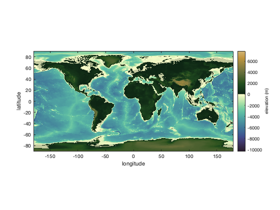
which contains the variables lat, lon, and Z. Plot them like this:

figure
imagesc(lon,lat,Z)
axis xy image
xlabel 'longitude'
ylabel 'latitude'
cb = colorbar;
ylabel(cb,'elevation (m)')
cmocean('topo','pivot')

Example 4: The effects of sea level rise

Let's take a quick look at the places that could be affected by sea level rise. Since we already loaded the full-resolution dataset in Example 3, we'll just use that dataset, except we'll begin by setting all ocean values to NaN. So make everything that's less than or equal to zero elevation NaN:

Z(Z<=0) = NaN;

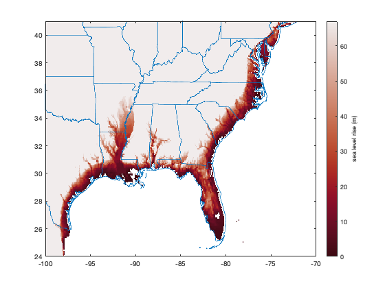
All the ice in Greenland and Antarctica holds the potential to raise global sea levels by about 67 m. Of course that scenario is not likely anytime soon, but let's look at the effects of such an event. We will have to make a crude (and incorrect) assumption that sea level would be distributed evenly around the present-day oceans, but it's a start.

To investigate the effects of adding about 67 m of sea level to the global ocean, plot the masked topography and set the color axis limits from 0 to 67 m:

figure
imagescn(lon,lat,Z)
caxis([0 67])
cb = colorbar;
ylabel(cb,'sea level rise (m)')
cmocean -amp % sets the colormap

To a first-order approximation, anywhere that's red is at risk of going underwater in the event of total collapse of the ice sheets. Darker red means more vulnerable. Let's zoom in on the eastern seaboard. Use the borders function to plot state boundaries.

axis([-100 -70 24 41])
borders('states')

A note on aliasing

The ETOPO5 dataset is provided at 5 minute (or 1/12 degree) resolution, but the topo_interp function does not do any anti-aliasing before interpolation. To meet the Nyquist requirement to prevent aliasing, you should technically interploate to grid points spaced at least twice the 5 minute resolution of the underlying dataset. That would be a very dense grid for the global dataset, so you may wish to accept a little bit of potential aliasing. Or you can load the raw data, use imresize to reduce the grid (while performing anti-aliasing) and interpolate. It's up to you.

Author Info

This function is part of the Climate Data Toolbox for Matlab. The function and supporting documentation were written by Chad A. Greene of the University of Texas at Austin.

topo_interp documentation

Contents